TR;DR
Linear regression gives you incorrect results when there exists
- Omitted variables bias
- Bad control
- Attenuation Bias This article explains them with Python examples.
(There are many other cases that gives you wrong regression results. This article only gives you three of them)
Omitted Variable Biases
Assume that you want to estimate how much additional one year of education increases one’s salary on average.
Your data has two variables: “years of education” and “salary”. You decided to regress them as:
Although you only have “educyear” in your variable, you realized that there exists an omitted variable “IQ” which affects obth “years of education” and “salary”.
While you don’t have “IQ” data, it seems people with high IQ tend to receive more education and higher salary.
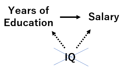
In this case, running a regression with just “educyear” will over/under-estimate educyear’s effect on salary.
Let’s see a Python example with a simulated data.
import numpy as np
import matplotlib.pyplot as plt
import statsmodels.api as sm
from mpl_toolkits.mplot3d import Axes3D
import plotly.graph_objects as go

# generate data
n = 300
x_iq = 100 + np.random.normal(0, 15, size=n)  # IQ is centered at 100 and have sd=15
x_educyear = np.random.randint(6, 10, n) + np.round(x_iq*0.1)  # Assume higher IQ leads to higher educyear
y_salary = 150 + 0.7*x_iq + 1.1*x_educyear + np.random.normal(0, 10, size=n)

# plot data
fig = go.Figure(data=[go.Scatter3d(x=x_iq, y=x_educyear, z=y_salary,
                                   mode='markers')])
fig.update_traces(marker_size=1)
fig.update_layout(scene = dict(xaxis_title='IQ',
                               yaxis_title='EducYear',
                               zaxis_title='Salary'),
                  margin=dict(l=0, r=0, t=0, b=0),)
fig.show()
Now estimate the coefficients.
X_modelA = np.column_stack((np.repeat(1, n), x_educyear))  # add y-intercept

ols = sm.OLS(y_salary, X_modelA)
ols_result = ols.fit()
print(ols_result.summary())
                            OLS Regression Results
==============================================================================
Dep. Variable:                      y   R-squared:                       0.462
Model:                            OLS   Adj. R-squared:                  0.460
Method:                 Least Squares   F-statistic:                     255.7
Date:                Tue, 05 Oct 2021   Prob (F-statistic):           5.52e-42
Time:                        12:18:32   Log-Likelihood:                -1180.1
No. Observations:                 300   AIC:                             2364.
Df Residuals:                     298   BIC:                             2372.
Df Model:                           1
Covariance Type:            nonrobust
==============================================================================
                 coef    std err          t      P>|t|      [0.025      0.975]
------------------------------------------------------------------------------
const        131.7647      6.902     19.090      0.000     118.181     145.348
x1             6.2147      0.389     15.990      0.000       5.450       6.980
==============================================================================
Omnibus:                        1.788   Durbin-Watson:                   1.784
Prob(Omnibus):                  0.409   Jarque-Bera (JB):                1.559
Skew:                          -0.081   Prob(JB):                        0.459
Kurtosis:                       3.314   Cond. No.                         172.
==============================================================================

Notes:
[1] Standard Errors assume that the covariance matrix of the errors is correctly specified.
The OLS regression result shows coefficient of 6.2147, although the true coefficient is 1.1.
Just in case, let’s test if we can estimate coefficients correctly when two variables are included.
X_modelB = np.column_stack((np.repeat(1, n), x_educyear, x_iq))
ols = sm.OLS(y_salary, X_modelB)
ols_result = ols.fit()
print(ols_result.summary())
                            OLS Regression Results
==============================================================================
Dep. Variable:                      y   R-squared:                       0.678
Model:                            OLS   Adj. R-squared:                  0.676
Method:                 Least Squares   F-statistic:                     313.1
Date:                Tue, 05 Oct 2021   Prob (F-statistic):           7.17e-74
Time:                        13:12:51   Log-Likelihood:                -1102.9
No. Observations:                 300   AIC:                             2212.
Df Residuals:                     297   BIC:                             2223.
Df Model:                           2
Covariance Type:            nonrobust
==============================================================================
                 coef    std err          t      P>|t|      [0.025      0.975]
------------------------------------------------------------------------------
const        144.9187      5.426     26.710      0.000     134.241     155.596
x1             0.9455      0.479      1.974      0.049       0.003       1.888
x2             0.7926      0.056     14.138      0.000       0.682       0.903
==============================================================================
Omnibus:                        0.131   Durbin-Watson:                   1.939
Prob(Omnibus):                  0.936   Jarque-Bera (JB):                0.027
Skew:                           0.007   Prob(JB):                        0.987
Kurtosis:                       3.044   Cond. No.                     1.02e+03
==============================================================================

Notes:
[1] Standard Errors assume that the covariance matrix of the errors is correctly specified.
[2] The condition number is large, 1.02e+03. This might indicate that there are
strong multicollinearity or other numerical problems.
For educyear, estimated=0.9455 vs true=1.1.
For iq, estimated=0.7926 vs true=0.7.
We can say that estimation is successful in this case.
To sum up, we need to always make sure we are not missing variables that affects both X and Y.
[Note] When we realized that there are omitted variable biases but we can’t collect missing variable, use Instrument Variable to obtain true coefficients.
Bad Control
In Omitted Variable Biases, we got a wrong result by NOT having the important variable.
In Bad Control, we get a wrong result by including unnecessary variables.
Assume again that you want to estimate the effect of “years of education” on “salary”.
You decided to regress “salary” with “years of education” and “number of pencils used in his/her life”.
Here, “number of pencils used in his/her life” is affected by “years of education” but has nothing to do with “salary”, as shown in the below graph.
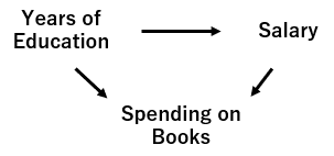
In this case, we should not include the irrelevant variable “number of pencils used” in the regression. What if we included in the regression model? Let’s see what will happen with Python example.
# generate data
n = 300
x_educyear = np.random.randint(6, 15, n)
y_salary = 150 + 8*x_educyear + np.random.normal(0, 10, size=n)  # x_book isn't there
x_book = 10*x_educyear + y_salary*0.6 + 10*np.random.randn(n)

# visualization
fig_2 = go.Figure(data=[go.Scatter3d(x=x_educyear, y=x_book, z=y_salary,
                                   mode='markers')])
fig_2.update_traces(marker_size=1)
fig_2.update_layout(scene = dict(xaxis_title='Educyear',
                                 yaxis_title='Books',
                                 zaxis_title='Salary'),
                    margin=dict(l=0, r=0, t=0, b=0),)
fig_2.show()
# OLS with full data
X_badcontrol = np.column_stack((np.repeat(1, n), x_educyear, x_book))  # add y-intercept
ols_bc = sm.OLS(y_salary, X_badcontrol)
ols_bc_result = ols_bc.fit()
print(ols_bc_result.summary())
                            OLS Regression Results
==============================================================================
Dep. Variable:                      y   R-squared:                       0.860
Model:                            OLS   Adj. R-squared:                  0.859
Method:                 Least Squares   F-statistic:                     909.8
Date:                Tue, 05 Oct 2021   Prob (F-statistic):          2.21e-127
Time:                        22:45:35   Log-Likelihood:                -1081.3
No. Observations:                 300   AIC:                             2169.
Df Residuals:                     297   BIC:                             2180.
Df Model:                           2
Covariance Type:            nonrobust
==============================================================================
                 coef    std err          t      P>|t|      [0.025      0.975]
------------------------------------------------------------------------------
const        110.8141      4.389     25.249      0.000     102.177     119.451
x1             1.3708      0.684      2.006      0.046       0.026       2.716
x2             0.4441      0.044     10.111      0.000       0.358       0.530
==============================================================================
Omnibus:                        1.719   Durbin-Watson:                   1.893
Prob(Omnibus):                  0.423   Jarque-Bera (JB):                1.503
Skew:                          -0.019   Prob(JB):                        0.472
Kurtosis:                       2.655   Cond. No.                     2.06e+03
==============================================================================

Notes:
[1] Standard Errors assume that the covariance matrix of the errors is correctly specified.
[2] The condition number is large, 2.06e+03. This might indicate that there are
strong multicollinearity or other numerical problems.
Although the true coefficient for x_educyear is 8, the OLS shows the coefficient of 1.3708.
Lesson: do not always include everything you have on your data.
You can check what are bad and good controls with this paper.
Attenuation Bias
Attenuation bias occures when there exists an observation error on x.
Assume that y is generated like below.
Assume also that we can only observe x-tilde, which is same as true x plus error:
n = 20

x1 = 100*np.random.rand(n)
y = 100 + x1*2 + np.random.normal(0, 10, size=n)

plt.figure(figsize=(10, 7))

plt.scatter(x1, y, marker='o', facecolors='none', edgecolors='blue', label='x-true')

# Add the bias term
X_modelA = np.column_stack((np.repeat(1, n), x1))

ols = sm.OLS(y, X_modelA)
ols_result = ols.fit()

plt.plot(x1, ols_result.predict(X_modelA), lw=1, color='blue')


###############################
nu = np.random.normal(0, 20, size=n)
x1_tilda = x1 + nu
plt.scatter(x1_tilda, y, marker='o', facecolors='none', edgecolors='red', label='x-tilda')

# Add the bias term
X_modelA = np.column_stack((np.repeat(1, n), x1_tilda))

ols = sm.OLS(y, X_modelA)
ols_result = ols.fit()

plt.plot(x1_tilda, ols_result.predict(X_modelA), lw=1, color='red')

arr = dict(shrink=0, width=0.1, headwidth=6,
                                headlength=10, connectionstyle='arc3',
                                facecolor='lightgray', edgecolor='lightgray')
for moto, ato, yy in zip(x1_tilda, x1, y):
    plt.annotate('', xy = (moto, yy), xytext = (ato, yy), color = "black", arrowprops = arr)

plt.legend(fontsize=15)

plt.show()
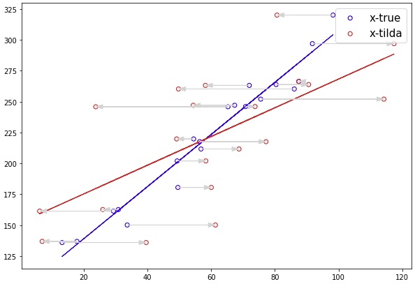
You can confirm the regression with x-tilda resulted in smaller coefficient. This is also called as regression dilution, the effect that biasing the regression coefficient towards zero.
References
- Angrist, Joshua D., and Jörn-Steffen Pischke. Mostly harmless econometrics. Princeton university press, 2008.